Tensors
TensorFlow에서 데이터의 중심 단위는 Tensor 입니다. Tensor는 다차원 배열의 primitive value 집합으로 구성됩니다. Tensor의 rank는 차원의 수를 의미합니다. 아래 예제가 있습니다.
3 # a rank 0 tensor; this is a scalar with shape []
[1. ,2., 3.] # a rank 1 tensor; this is a vector with shape [3]
[[1., 2., 3.], [4., 5., 6.]] # a rank 2 tensor; a matrix with shape [2, 3]
[[[1., 2., 3.]], [[7., 8., 9.]]] # a rank 3 tensor with shape [2, 1, 3]
여기서 primitive value는 숫자나 문자열 같은 원시적인 값들을 의미합니다.
TensorFlow Core tutorial
Importing TensorFlow
TensorFlow 프로그램에 대한 표준 import 방법은 다음과 같습니다.
import tensorflow as tf이렇게 하면 python에서 TensorFlow의 모든 class, method 및 symbol을 access 할 수 있습니다. as tf는 tensorflow라는 모듈 이름이 길기 때문에 tf로 사용하겠다는 의미입니다.
The Computational Graph
TensorFlow Core 프로그램은 두 개의 섹션으로 구성되어 있다고 할 수 있습니다.
- computational graph 빌드
- computational graph 실행
Computational graph는 일련의 TensorFlow 작업을 node graph로 배열한 것 입니다. 간단한 computational graph를 작성해 봅시다. 각 node는 0 이상의 tensor를 입력으로 받으며, 출력으로써 tensor를 생성합니다. constant는 node의 type중 하나 입니다. TensorFlow의 constant도 일반적인 constant와 마찬가지로 입력을 받지 않고 내부적으로 저장된 값을 출력합니다. 다음과 같이 두 개의 floating point형 tensor node1과 node2를 만들 수 있습니다.
node1 = tf.constant(3.0, tf.float32)
node2 = tf.constant(4.0) # also tf.float32 implicitly
print(node1, node2)
여기서 자료형을 명시하지 않으면 floating point형에 대해서 default값으로 float32 자료형이 설정되는 듯 합니다.
마지막 print 문의 결과는 다음과 같습니다.
Tensor("Const:0", shape=(), dtype=float32) Tensor("Const_1:0", shape=(), dtype=float32)
sess = tf.Session()
print(sess.run([node1, node2]))
우리의 예상과 같이 3.0과 4.0을 볼 수 있습니다.
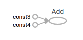
[3.0, 4.0]tensor node를 operation과 결합하여 좀 더 복잡한 계산을 할 수 있습니다(operation 또한 node 입니다). 예를 들면, 두 개의 constant node를 add하고 다음과 같이 새로운 graph를 생성할 수 있습니다.
node3 = tf.add(node1, node2)
print("node3: ", node3)
print("sess.run(node3): ",sess.run(node3))
print 두 줄의 결과는 다음과 같습니다.
node3:  Tensor("Add_2:0", shape=(), dtype=float32)
sess.run(node3):  7.0
첫 번째 print 결과는 node를 session 내에서 실행하지 않았기 때문에 tensor의 속성이 출력 되었습니다.
TensorFlow는 TensorBoard라고 불리는 utility를 제공합니다. 이는 computational graph를 그림으로 나타낼 수 있습니다. 다음은 TensorBoard가 graph를 시각화 하는 방법을 보여주는 스크린샷 입니다.
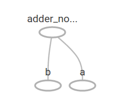
placeholder는 외부 입력을 허용하도록 graph를 매개변수화 할 수 있습니다. placeholder는 값을 나중에 변경할 수 있습니다.
a = tf.placeholder(tf.float32)
b = tf.placeholder(tf.float32)
adder_node = a + b  # + provides a shortcut for tf.add(a, b)
두 개의 입력 매개변수(a와 b)를 정의하고 이들에 대한 연산을 정의합니다. feed_dict 매개변수를 사용하여 placeholder에 값을 입력할 수 있습니다.
print(sess.run(adder_node, {a: 3, b:4.5}))
print(sess.run(adder_node, {a: [1,3], b: [2, 4]}))
결과는 다음과 같습니다.
7.5
[ 3.  7.]
TensorBoard에서는 다음과 같이 표현됩니다.
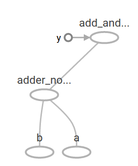
다른 operation을 추가하여 computational graph를 좀 더 복잡하게 만들 수 있습니다. 예를 들면,
add_and_triple = adder_node * 3.
print(sess.run(add_and_triple, {a: 3, b:4.5}))
결과는 다음과 같습니다.
22.5이 computational graph는 TensorBoard에서 다음과 같이 표현됩니다.
머신러닝에서 우리는 일반적으로 위와 같은 임의의 입력을 받을 수 있는 model을 원할 것입니다. model을 학습 가능하게 만들려면 동일한 입력으로 새로운 출력을 얻기 위해 graph를 수정할 수 있어야 합니다. Variable을 사용하면 graph에 학습 가능한 매개변수를 추가할 수 있습니다. Variable은 타입과 초기값으로 구성됩니다.
W = tf.Variable([.3], tf.float32)
b = tf.Variable([-.3], tf.float32)
x = tf.placeholder(tf.float32)
linear_model = W * x + b
여기서 [.3]은 0.3을 [-.3]은 -0.3을 의미합니다.
constant는 tf.constant를 호출할 때 초기화 되며 값은 절대로 변경될 수 없습니다. 이와 반대로, tf.Variable을 호출하면 variable이 초기화되지 않습니다. TensorFlow 프로그램의 모든 variable을 초기화하려면 다음과 같이 특별한 operation을 명시적으로 호출해야 합니다.
init = tf.global_variables_initializer()
sess.run(init)
여기서 init은 모든 global variable을 초기화하고 있습니다. sess.run을 호출하기 전까지는 variable은 초기화되지 않습니다. x는 placeholder이므로, 다음과 같이 x의 여러 값에 대해 linear_model을 동시에 evaluate할 수 있습니다.
print(sess.run(linear_model, {x:[1,2,3,4]}))결과는 다음과 같습니다.
[ 0. 0.30000001 0.60000002 0.90000004]우리는 model을 만들었지만 이 model이 얼마나 좋은지는 알 수 없습니다. training data에 대해 model을 evaluate해야 합니다. 이는 목표 값을 제공하기 위해 y placeholder가 필요하며, loss function을 추가해야 합니다. 여기서 y는 training data set을 의미합니다. loss function은 cost function과 같은 의미입니다.
loss function은 제공된 data로부터 현재 model이 얼마나 떨어져 있는지를 측정합니다. 표준 loss model인 linear regression을 사용합니다. linear regression은 현재 model과 제공된 data 사이의 delta 제곱을 더해서 계산합니다. linear_model - y는 각 요소가 error delta인 vector를 만듭니다. tf.square를 호출하여 error를 제곱합니다. 그런 다음 모든 제곱 error를 합산하여 단일 scalar를 만듭니다. 이 과정은 tf.reduce_sum을 사용하여 계산할 수 있습니다. training data와 설계한 linear_model과의 차이의 제곱의 합을 계산합니다.
y = tf.placeholder(tf.float32)
squared_deltas = tf.square(linear_model - y)
loss = tf.reduce_sum(squared_deltas)
print(sess.run(loss, {x:[1,2,3,4], y:[0,-1,-2,-3]}))
loss 값은 다음과 같습니다.
23.66W와 b의 값을 -1에서 1의 값으로 재할당하여 수동으로 향상시킬 수 있습니다. variable은 tf.Variable을 사용하여 제공된 값으로 초기화 되지만, tf.assign operation을 사용하여 변경할 수 있습니다. 예를 들면, W=-1, b=1은 우리 model에 대한 최적의 매개변수 입니다. 이에 따라 W와 b를 변경할 수 있습니다.
fixW = tf.assign(W, [-1.])
fixb = tf.assign(b, [1.])
sess.run([fixW, fixb])
print(sess.run(loss, {x:[1,2,3,4], y:[0,-1,-2,-3]}))
마지막 print는 loss가 0임을 보여줍니다.
0.0우리는 W와 b의 "완벽한" 값을 추측하고 적용하였습니다. 그러나 머신러닝의 요점은 올바른 model의 매개변수를 자동으로 찾는 것 입니다. 다음 섹션에서 이를 수행하는 방법을 보여줍니다.
여기까지 실행 결과 입니다.

소스 코드도 첨부하였습니다.
 PythonApplication1.py
출처
'머신러닝 > TensorFlow' 카테고리의 다른 글
| tf.contrib.learn (0) | 2017.03.08 |
|---|---|
| tf.train API (0) | 2017.03.07 |
| 설치하기 (2) | 2017.02.21 |
| TensorFlow란? (0) | 2017.02.21 |